The strange origins of the Student’s t-test

Features

Angus Brown
University of Nottingham, Nottingham, UK

---

https://doi.org/10.36866/pn.71.13

The centenary of the introduction of the Student’s t-test may not be as auspicious an anniversary as some, but the Student distribution around which the t-test is based has had an impact on experimental design and sampling theory far in excess of the modest intentions of its originator, William Sealy Gosset (Fig. 1). In order to fully appreciate the impact of the Student’s t-test on modern biostatistical analysis we must travel back over a century to assess the current statistical trends of the day.

At the onset of the 20th century statistical analysis was dominated by the concepts of populations and very large sample numbers, whose chief advocate was Karl Pearson. The central core of such analysis was the normal distribution, which was first derived by de Moivre in 1733 (de Moivre, 1738) to predict the outcome of games of chance, and later, based on the application of the distribution to astronomical analysis, expressed as a probability frequency distribution (equation 1) by Gauss:

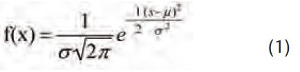
where σ is the standard deviation, and μ is the mean. A large number of parameters/characteristics in biology are accurately described by a normal distribution (Fig. 2), which has the following characteristics:

• it is symmetrical about the centre, with this as the point containing the highest frequency;
• the mean, median and mode are the same;
• the inflexion of the curve is ± 1 standard deviation (SD) from the centre (mean);
• the tails asymptote towards zero;
• the means of large groups of samples (n > 120) from within a population described by a normal distribution, will also be normally distributed (note that this is not the case for smaller groups of samples, the catalyst that impelled Gosset to establish his
  ‘ Student’s t’distribution).

Since biological parameters of populations are accurately described by a normal distribution, it follows that the properties of the normal distribution can be applied to these parameters. The key characteristic of a normal distribution is that the area under the curve, which equates to the proportion of data lying between two points, can be defined in terms of SDs relative to the mean. Thus 68% of the area is contained within ± 1 SD of the mean, 95% of the area is contained within ± 1.96 SD of the mean, and 99% of the area is contained within ± 2.56 SD of the mean (Fig. 2). This ability to accurately define the distribution of data relative to the SD led to the concept of confidence limits, where the probability that data will lie between distinct SD spans can be stated as a percentage. For example, there is a 95% probability that a data point for any normal distribution will lie between ± 1.96 SD of the mean. The normal distribution can also be used to make inferences about data from two sample groups. If the mean of one sample group lies between the 95% confidence limits of the other sample group, there is only a 5% chance that the two sample groups are not drawn from the same population. This is a key relationship, as we shall soon see.

It is at this point that William Sealy Gosset enters the picture. Born in Canterbury in 1876, Gosset was educated at Winchester and Oxford, where he obtained a first in chemistry in 1897 and a first in mathematics in 1899. He was hired by the Guinness brewery in Dublin, in whose employ he spent the remainder of life, mainly at St James Gate in Dublin, and for the final 2 years at Park Royal, London. Gosset’s academic background may seem at odds with his employment as a brewer, but Guinness realized around this time that in order to maintain its dominant market share as the biggest brewer in Ireland, it would have to introduce brewing on a carefully controlled industrial scale. Such a venture would require rigorous quality control; hence the requirement for university trained chemists and statisticians. As any amateur brewer will attest, the brewing of beer has an element of the unknown, with success being not only dependent on the correct procedure, but also an element of luck! It was this reliance on luck for a successful product that Guinness sought to eliminate by scientific procedure. Beer, of course, is a combination of natural products; malted barley, hops and yeast, all mixed with water. These natural products share an inherent variability common to all agricultural products, whose quality is dependent not only upon crop variety, but also on climate, soil conditions, etc. Gosset’s task as Apprentice Brewer was not only to assess the quality of these products, but also to do so in a cost effective manner. This necessitated using experiments with small sample numbers to draw conclusions that could be applied to the large scale brewing process. However, Gosset discovered that in using small samples the distribution of the means deviated from the normal distribution. He therefore could not use conventional statistical methods based upon a normal distribution to draw his conclusions.

In 1904 Gosset published an internal report entitled The application of the ‘ Law of Error’ to the work of the brewery, where he described how ‘the greater the number of observations of which means are taken, the smaller the (probable) error’. Gosset also noted how, compared to a normal distribution, ‘the curve which represents their frequency of error becomes taller and narrower’ as sample size decreases (Fig. 2, black line). The Guinness management realized the potential cost savings impact of the study and suggested Gosset consult with a professional mathematician.

Gosset therefore wrote to Karl Pearson at UCL, and they met on 12 July 1905 while Gosset was on holiday in England. This meeting led to an invitation for Gossett to visit Pearson’s department at UCL in 1906/07 for a year, where he worked on his small samples problem. In 1908 Gosset published the fruit of his labours in a paper entitled The probable error of a mean in the journal Biometrica (Student, 1908), of which Pearson was Editor. However, Guinness had a policy of not publishing company data, and allowed Gosset to publish his observations on the strict understanding that he did so anonymously, and did not use any of the company’s data. Gosset complied and published under the pseudonym ‘Student’ – the name under which he would publish 19 of his 21 publications. The name Student apparently came from the cover of a notebook Gosset used at the time – The Student’s Science Notebook (Ziliak, 2008).

In his classic paper Gosset states that ‘any series of experiments is only of value is so far as it enables us to form a judgment as to the statistical content of the population to which the experiment belongs.’ Or, stated another way – having n observations Gosset wanted to know within what limits the mean of the sampled population lay. In the paper Gosset partially derives the distribution of the error (termed z) and gives values of z from n = 4 to 10. This table is expressed as a cumulative distribution function (Fig. 2, inset) relative to n and z. The calculations required to generate the table of z values were very labour-intensive and took Gosset about 6 months to compute on a mechanical calculator, bringing to mind an equivalent labour carried out by Andrew Huxley in the mathematical reconstruction of the squid axon action potential
(Hodgkin & Huxley, 1952). Gosset concluded the paper with several examples in which he computed the odds of a variety of scenarios occurring. To do this he simply divided the difference of the means by the standard deviation to calculate z, and then looked up the tables at the appropriate level of n. The cumulative distribution function was then converted to odds. The higher the value of z, then the greater the likelihood that the conclusions drawn from the test were correct. An essential component of the Student distribution is that, as the value of n decreases, so does the cumulative distribution function at the same value of z. Or, as we shall soon see, according to Fisher’s argument the smaller the value of n the greater the value of t at the same probability (Fig. 3). This translated the familiar experimental scenario where the smaller the n value, the greater the difference between the two samples required in order to achieve any particular level of significance (Fig. 4). Such phrases as ‘and in practical life such a high probability is in most matters considered a certainty’, ‘but would occasion no surprise if the results were reversed by further experiments’ and ‘would correspondingly moderate the certainty of his conclusion’ (Student, 1908), indicate the importance that Gosset put on the intuition of the individual experimenter or statistician in determining the meaning of the result. Gosset continued to use his table of z distribution in the course of his work, but otherwise it was ignored.

In 1912 Gosset communicated with a young statistician, Ronald Fisher, who would have an enormous impact on the acceptance of Student’s distribution in day-to-day statistical analysis. Fisher is known today as one of the founding fathers of modern biostatistics, and he was not slow to appreciate Gosset’s contribution. In 1917 Gosset published an extended table of z distribution for n = 2 to 30, stating of the table of z values in his 1908 paper ‘I stopped at n = 4 because I had not realized that anyone would be foolish enough to work with probable errors deduced from a smaller number of observations’ (Student, 1917). Some years later In 1925 Fisher published a paper in which he fully derived the values of Student’s distribution, his final distribution being equivalent to the form given by Gosset in 1908, and clearly showing it as a transformed normal distribution (Fisher, 1925). In this seminal paper Fisher also provided a worked example with two groups of unequal sample number. Fisher changed the nomenclature of the distribution from z, as it appeared in Gosset’s original paper, to t, and changed the distribution from n to (n – 1) or degrees of freedom (df). On this amendment Gosset commented thus: ‘When you only have quite small numbers, I think the formula we used (incorporating n – 1) is better, but if n be greater than 10 the difference is too small to be worth the extra trouble’ (Pearson, 1939). Pearson was skeptical, stating his contention that the number of samples should be large enough that n – 1 is indistinguishable from n. This reflected his continued resistance to the use of small sample numbers. However, Fisher must have exerted an influence at an early stage, as by 1917 Gosset was using (n – 1) in his extension of the table of z distributions (Student, 1917). Fisher also transformed the layout of Student’s distribution to fit with his own agenda, namely to promote the use of probability as a determining factor in such calculations (Ziliak & McClosky, 2008). In Fisher’s table the t value is expressed relative to p (probability) and df. Thus for a given df and desired probability the t value is located, and if this value is greater than the computed t value based on experimental data, then there is no significant difference in the data at that probability. This was certainly not how Gosset pictured his z distribution being used, but Fisher was an extremely eloquent and powerful advocate who rapidly came to dominate the field, and it is his form of the calculation that we use today (Rohlf & Sokal, 1995).

Gosset himself had no academic pretensions, and he comes across as a pragmatic man. He was dismissive about his mathematical ability, stating that the limits of his capabilities ‘stopped at Maths, Mods [final examinations] at Oxford, consequently I have no faculty therein’ (Gosset, 1962). Gosset was clearly nobody’s fool, but his mathematical skills were not on a par with Fisher or Pearson. That his derivation of t was incomplete and partly guessed bears out this point, but Fisher’s fully derived t distribution of 1925 showed Gosset’s intuition to be correct. Indeed Fisher comments ‘any capable analyst could have shown him the demonstration he needed’. Gosset’s calculations frequently contained minor errors and he preferred to do his calculations on the backs of envelopes and scraps of paper (McMullen, 1939), an endearing amateurism only reinforced by comments such as ‘In a similar tedious way we find’ during an extended derivation (Student, 1908). However, the t distribution allowed Gosset to proceed with his work for Guiness, and he was promoted to head experimental brewer and head of statistics, and finally in 1935 promoted to Head Brewer, a position he held until his death 2 years later.

This is a brief history of the introduction of Student’s t distribution, but how is it applied in the Student’s t–test? The first step in this calculation is to determine the value of t for the given df and level of probability which, for our purposes, we will take as 0.05 (5%). Given the t distribution we can then calculate the confidence limits from the mean and SD of the sample groups (the t-test requires that both groups have the same variance and are normally distributed). Plotting these on a graph allows us to visually assess the data. If the mean of Group 2 falls outside of the upper and lower 95 %confidence limits (i.e. outside the confidence interval) of Group 1, then there is less than a 5% chance that the Group 2 data are from the same population as Group 1 (Fig. 4). It would be rather tedious to plot a graph of the data each time we wanted to compare two groups, but the graph can be reduced to a simple equation (equation 2).

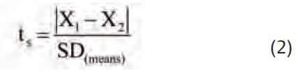
where X1 and X2 are the means of the two groups, and the vertical lines are an indication to subtract the smaller value from the larger. In this equation ts is calculated based on the experimental data. If ts exceeds the t value for the appropriate df and probability (i.e ts > t) then the two groups are different at that level of probability.

It should be fairly easy to see from Fig. 4 the logic of the equation. The greater the value of ts the more likely the two groups are to be drawn from different populations, irrespective of df. The greater the difference between X1 and X2, or the smaller the SD (means) the greater the value of ts. There are numerous spreadsheet examples of t-test calculations, which are worth doing once to see the workings of the equation, but are superfluous for day-to-day calculations since spreadsheets programmes such as Microsoft Excel have built in t-test functions, and the above equation only yields a ts value, not the exact p values, which cannot easily be calculated.

In conclusion, physiologists (and many other experimental scientists) owe Gosset a debt of gratitude for rendering obsolete the reliance on large sample sizes to determine differences between groups of data. The t-distribution allows experimenters the freedom to use small sample sizes in the confidence that they are not compromising the validity of any conclusions drawn: indeed the Home Office policy of Reduction, Refinement and Replacement with regard to animal experiments would be impossible without the t-distribution.

That Gosset, surely the unsung hero of 20th century statistics, made such an enormous advance in the field of statistics is almost certainly due to his application of theory to solve practical problems. In a letter to Fisher regarding his t distributions Gosset lamented that ‘you are the only man that’s ever likely to use them’. A browse through any issue of The Journal of Physiology will serve to illustrate the ubiquity of Student’s t test in the life sciences, and demonstrate just how unaware Gosset was of the revolutionary impact his work would have on all fields of biology and beyond.

References

de Moivre (1738). The doctrine of chances, 2nd edn.

Fisher R A (1925). Applications of ‘Student’s’ distribution. Metron 5, 90-104.

Gosset W S (1962). Letter No 2 to R A Fisher. Guinness Son & Co Ltd, Dublin. Private Collection.

Hodgkin A & Huxley A (1952). A quantitative description of membrane current and its application to conduction and excitation in nerve. J Physiol 117, 500–544.

McMullen L (1939). ‘Student’ as a man. Biometrika 30, 204-210.

Pearson E S (1939). ‘Student’ as statistician. Biometrika 30, 210-250.

Rohlf F J & Sokal R R (1995). Statistical tables. In Biometry: the principles and practice of statistics in biological research, 3rd edn, p. 199. W H Freeman & Co, New York.

Student (1908). The probable error of a mean. Biometrika 4, 1-24.

Student (1917). Tables for estimating the probability that the mean of a unique sample of observations lies between -∞ and any given distance of the mean of the population from which the sample is drawn. Biometrika XV, 414-417.

Ziliak S T & McCloskey D N (2008). In The cult of statistical significance, p. 352. University of Michigan Press, Michigan.

Ziliak S T (2008). The great skew: R A Fisher and the copyright history of ‘Student’s’ t. http://faculty.roosevelt.edu/Ziliak.