Rasmus Dahl, University of Copenhagen, Denmark

Ronan Berg, University of Copenhagen, Denmark

https://doi.org/10.36866/pn.120.25

Electrocardiography is a method used to measure the electrical activity of the heart in order to detect cardiac disease. The cardiac conduction system synchronises the pumping action of the heart, and during cardiac contraction a spike in the electrical current represented by the QRS complex on the electrocardiogram is observed due to depolarisation of cardiomyocytes. The direction of this net current is termed the “mean electrical axis of the heart”, which is a mandatory topic in almost any undergraduate course on cardiac electrophysiology, and which may be used clinically to detect hypertrophy, cardiac conduction disturbances, and the origin of arrhythmias.

As with many other physiological concepts that are strictly mathematical, the mean electrical axis of the heart is a somewhat divisive topic among undergraduate students. Some find it intuitive while others do not. Thus, when teaching this topic, a firm outline of the underlying trigonometric principles may either be an eye-opener (“ah, now I get it, it’s all just about triangles!”) or cause even more confusion (“you have completely lost me now – what do triangles have to do with anything?”). In any event, the mean electrical axis of the heart is indeed all about triangles, and in the present paper, we use the underlying trigonometric principles to derive a general equation that permits the determination of the mean electrical axis of the heart from any two limb leads in a quick and easy manner. Although this approach will not be suitable for all students, it may unveil the wonders of cardiac electrophysiology to those who find mathematics intuitive.

What is “the mean electrical axis of the heart”?

The concept of a mean electrical axis of the QRS complex in the ECG was first introduced by Willem Einthoven in 1913 (Einthoven et al., 1913), and to this day it remains a clinically important aspect of ECG diagnostics. It represents the average direction of the ventricular depolarisation wave in the frontal plane, that is, the total vector of all the depolarisations that occur throughout the ventricles during the cardiac cycle. It is represented graphically in a triaxial system, the so-called “circle of axes” (Fig. 1).

According to the concept of a mean electrical axis of the heart, the centre of the heart is assumed to be located at the centre of the “circle of axes”, the triangles formed by the bipolar (I, II, and III) and augmented unipolar (aVL, aVR, and aVF) limb leads are assumed to be equilateral, and the thorax is assumed to be a homogeneous conductor. In the “circle of axes” the equilateral triangle of the bipolar leads is visualised by the vector sum of lead I and lead III, which is equal to lead II. The equilateral triangle of the augmented unipolar leads is constructed by connecting the head of vectors in the “circle of axes” (Fig. 1).

Obviously, none of these assumptions are entirely valid in vivo, but the mean electrical axis nonetheless provides information on the state of intraventricular conduction, as well as left vs. right ventricular muscle mass. The electrical axis of the heart is normally between -30˚ and +90˚, and may vary by up to 35˚ during normal breathing due to the associated movements of the heart (Moody et al., 1985). An electrical axis between -30˚ and -90˚ is coined left axis deviation, while right axis deviation is defined as an electrical axis between +90˚ and +180˚. During normal sinus rhythm without bundle-branch block, left axis deviation may notably be caused by left anterior fascicular block, left ventricular hypertrophy and/or fibrosis, while left posterior fascicular block and right ventricular hypertrophy may cause right axis deviation. Fascicular blocks occur when electrical activity of either the anterior or posterior fascicle of the left bundle branch is delayed or blocked. Furthermore, assessment of the mean electrical axis may be an aid for identifying the origin of some arrhythmias, notably so-called broad complex tachycardias.

The “circle of axes” vs. the “Novosel formula”

The abovementioned “circle of axes” is typically used to graphically derive the mean electrical axis of the heart by plotting the net voltage of the QRS complex in two bipolar limb leads (Carter, 1919). A line that is perpendicular to the respective lead axis is drawn through each mark, and the centre of the circle of axes (tail of vector) is connected to the intersection point between these two lines (head of vector) to form the cardiac vector. The mean electrical axis is then measured as the angle of this position vector (Fig. 2).

The underlying trigonometric principles also permit an alternative equation-based approach, so that the mean electrical axis may be determined from any two limb leads, including both the bipolar and augmented unipolar limb leads. The derivation of a general equation for the mean electrical axis is available as an online supplement to this article. Several specific formulas may be derived from this, and the combination of lead I (V_I) and aVF (V_aVF) yields the following formula:

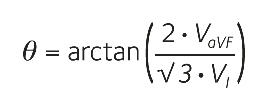
where θ is the mean electrical axis of the heart. Incidentally, this specific equation has previously been derived on an entirely different basis (Novosel et al., 1999), and we therefore designate it the ‘Novosel formula’. In Fig. 3 this formula is used to derive the mean eletrical axis in three ECGs with normal axis, left axis deviation and right axis deviation.

Figure 3. The mathematical method for determining the mean electrical axis of the heart. Examples of ECGs with normal electrical axis, left axis deviation, and right axis deviation. The mean electrical axis can be calculated by the Novosel formula using the net QRS voltages in leads I and aVF. For the ECG with left axis deviation, we find VI = 0.5 mV – 0.1 mV = 0.4 mV and VₐVF = 0.4 mV – 1.0 mV = –0.6 mV. By insertion into the formula we get: tan(θ) = –1.73. This equation has two solutions in the interval from 0˚ to 360˚, which are θ₁ = –60˚ and θ₂ = 120˚. The mean eletrical axis always has the same sign as the net QRS voltage in aVF, thus the result is θ = –60˚. The same method can be used to calculate the normal axis (VI = 0.8 mV, VₐVF = 0.8 mV, θ = 49˚) and right axis deviation (VI = –0.3 mV, VₐVF = 1.1 mV, θ

Conclusion

Good teaching is all about knowing your audience, and a strictly mathematically based approach like this one is probably not suitable for most physiology lecture settings. Outside lectures, it may nonetheless be used as an extracurricular tool to unveil the wonders of cardiac electrophysiology to interested students that find mathematics intuitive. Furthermore, the ‘Novosel formula’ presented here provides a much easier and quicker means for determining the mean electrical axis of the heart than the “circle of axes” and may thus be of use in the clinical setting.

For more information, please read this online supplement.