https://doi.org/10.36866/pn.123.8

Dr Dragutin Novosel
Matija Alanović
Robert Žunac
Dr Tina Bečić

In a recent publication, Dahl and Berg (2020) discussed teaching the principles of the mean electrical axis of the heart (EA) from standard electrocardiogram (ECG) recordings, its background, its underlining physiological processes and its trigonometry, which were accompanied by an illustrated, typical case. The authors explained the historical background and development of the calculation of the EA, including its clinical applications, graphical representations, and difficulties in its teaching, and they referenced a formula published previously by us (Novosel et al., 1999). Furthermore, Dahl and Berg (2020) discussed future perspectives from an educational-methodological point of view. Their descriptions were clear-cut and instructive. Additionally, they accentuated the differences between the theoretical assumptions of the EA and how it is performed in practice. However, we would like to emphasise three topics: (i) the relationships between the limb leads; (ii) the visualisation of the ‘Novosel Formula’; and (iii) the lack of standardisation when calculating the EA.

Relationships between limb leads

The standard (bipolar) ECG limb leads are named as I, II and III. The augmented (unipolar) leads are described as aVR, aVL and aVF. As delineated elsewhere (Novosel et al., 1999, Dahl and Berg, 2020), basically, from any two known leads, any other lead can be calculated: for example, aVR = aVL-1.5*I. The EA can be calculated or graphically estimated from a combination of any two limb leads. Mostly, the EA is calculated or grapically estimated from leads I/II of I/aVF (Dahl and Berg, 2020). However, the EA can be calculated, e.g. from leads III and aVR as EA = ± ArcTan [2 / √3 * (0.75*III-0.5*aVR)/(-0.5*III-aVR)], but the delineation and listings of all formulas are beyond the scope of the current paper. The argument is for at least having access to all mathematical relationships between limb leads and different calculations of the EA results when a manual measurement of the QRS amplitude is needed; therefore, it makes sense to take the two leads with the highest amplitudes to calculate the EA. The error of the manual measurement is relatively lower if the amplitudes are high compared with lower amplitudes. As a consequence, we propose using the leads with the highest amplitudes to estimate the EA.

Visualisation of the Novosel Formula

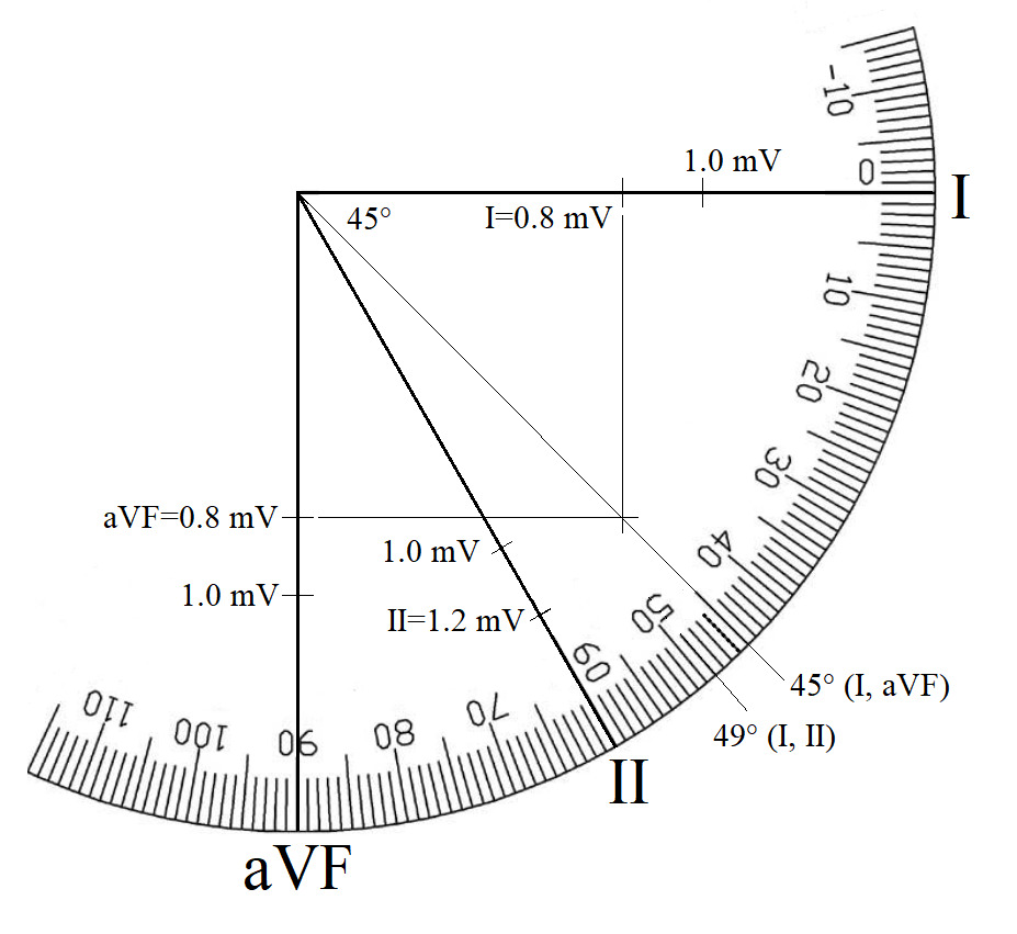
With the permission of Dahl and Berg, we modified their original figure (Dahl and Berg, 2020) and used their sample of a normal ECG. For the purpose of this publication we are using only the right-down quadrant. They estimated the value of lead I as 0.8 mV and the value of the aVF as 0.8 mV. Correspondingly, the value of the lead II is 1.2 mV. Fig. 1 shows a graphical representation provided by Dahl and Berg of the EA as estimated from a combination of leads I and II. Fig. 2 shows a graphical representation of the EA as estimated from leads I and aVF without correction of the lead aVF. Fig. 3 (the visualisation of the ‘Novosel Formula’) shows a graphical representation of the EA as estimated from a combination of leads I and II (as shown in Fig. 1) plus a combination of leads I and the recalculated value of aVF (Novosel et al., 1999; the recalculated aVF = 2*aVF/√3).

It is important to note that graphical determination of the EA from leads I/II and leads I/aVF with the correction are identical (also to numerical estimation as described elsewhere, Novosel et al., 1999), whereas the graphical determination of the EA from leads I/aVF without correction (as frequently used in teaching and demonstrations) results in a different (and incorrect) value. The explanation for this error is that the augmentation factor of leads I, II and III (bipolar leads) is different when compared with (unipolar) leads aVR, aVL and aVF (Dahl and Berg, 2020) as recorded and calculated by the ECG device itself due to the mathematical relationships of the leads.

Conclusively, any combination of leads I/II/ III or aVR/aVL/aVF separately can be used without any corrections to estimate the EA; however, when a combination of bipolar and unipolar leads is used to calculate the EA, the correction must be made. The differences will seldom reach any clinical significance and are of pure methodological value but may play a significant role in large-scale research and “deep-data” analysis (Wagner et al., 2020).

Absence of standardisation

There are clear and precise recommendations for standardising and interpreting an ECG, including estimating of the normal EA and its deviations (Kligfield et al., 2007; Mason et al., 2007). Even this comprehensive publication neglected to standardise how the EA should be calculated. However, to the best of our knowledge, ECG devices available on the market calculate the EA using different rules. Some ECG devices use the value of a single QRS complex, and some calculate the mean of several QRS complexes and use these mean values to calculate the EA. These EA values could be named as “mean of the mean of the EA”. Some devices use leads I and II, whereas others use leads I and aVF (with or without correction). Despite minimal significance in a single case, the results are not amenable to large-scale research as the assessments/calculations do vary. Therefore, we propose the development of a standard for calculating the mean EA.

Conclusion

As recently discussed by Dahl and Berg, there are different factors that should be considered regarding the issue of calculating the EA: theoretical aspects, teaching, rapid measurements in a clinical setting, electrocardiographic device-driven estimation and, as added by use, the standardisation. Certainly, these issues do overlap. Although the standardisation of the calculation of the mean electrical axis may not play any role in basic education and in a clinical, single-case setting, there is a need to standardise the calculation for electrocardiographic devices. Standardisation of the algorithms in electrocardiographic devices gains importance not only in large-scale, multi-centric studies, which inevitably include different devices, but also because of the “big-data” approach now being increasingly used. Standardisation would enable more precise analyses, comparisons, reproducibility and reductions in unnecessary variability caused by the use of different formulas.

References

Dahl R and Berg R (2020). Trigonometry of the ECG. A formula for the mean electrical axis of the heart. Physiology News 120, 25-27.

Kligfield P et al. (2007). Recommendations for the standardization and interpretation of the electrocardiogram Part I: The electrocardiogram and its technology. Circulation 115, 1306-1324.

Mason JW et al. (2007). Recommendations for the standardization and interpretation of the electrocardiogram Part II: Electrocardiography diagnostic statement list. Circulation 115, 1325-1332.

Novosel D et al. (1999). Corrected formula for the calculation of the electrical heart axis. Croatian Medical Journal 40, 77-79.

Wagner P et al. (2020). PTB-XL, a large publicly available electrocardiography dataset. Scientific Data 7, 154-160.